In class exercise network

Published

March 8, 2024

Modified

March 16, 2024

Load packages:

pacman::p_load(igraph,tidygraph, ggraph, visNetwork,lubridate,clock,tidyverse,graphlayouts)

Importing network data from files

GAStech_nodes <- read_csv("data/GAStech_email_node.csv")
GAStech_edges <- read_csv("data/GAStech_email_edge-v2.csv")

create 2 more columns

GAStech_edges <- GAStech_edges %>%
  mutate(SendDate = dmy(SentDate)) %>%
  mutate(Weekday = wday(SentDate,
                        label = TRUE,
                        abbr = FALSE))

Wrangling attributes

A close examination of GAStech_edges data.frame reveals that it consists of individual e-mail flow records. This is not very useful for visualisation.

In view of this, we will aggregate the individual by date, senders, receivers, main subject and day of the week.

GAStech_edges_aggregated <- GAStech_edges %>%
  filter(MainSubject == "Work related") %>%
  group_by(source, target, Weekday) %>%
    summarise(Weight = n()) %>%
  filter(source!=target) %>%
  filter(Weight > 1) %>%
  ungroup()

Using `tbl_graph()` to build tidygraph data model.

In this section, you will use tbl_graph() of tinygraph package to build an tidygraph’s network graph data.frame.

Before typing the codes, you are recommended to review to reference guide of tbl_graph()

GAStech_graph <- tbl_graph(nodes = GAStech_nodes, edges = GAStech_edges_aggregated, directed = TRUE)

GAStech_graph %>%
  activate(edges) %>%
  arrange(desc(Weight))

# A tbl_graph: 54 nodes and 1372 edges
#
# A directed multigraph with 1 component
#
# Edge Data: 1,372 × 4 (active)
    from    to Weekday   Weight
   <int> <int> <ord>      <int>
 1    40    41 Saturday      13
 2    41    43 Monday        11
 3    35    31 Tuesday       10
 4    40    41 Monday        10
 5    40    43 Monday        10
 6    36    32 Sunday         9
 7    40    43 Saturday       9
 8    41    40 Monday         9
 9    19    15 Wednesday      8
10    35    38 Tuesday        8
# ℹ 1,362 more rows
#
# Node Data: 54 × 4
     id label           Department     Title           
  <dbl> <chr>           <chr>          <chr>           
1     1 Mat.Bramar      Administration Assistant to CEO
2     2 Anda.Ribera     Administration Assistant to CFO
3     3 Rachel.Pantanal Administration Assistant to CIO
# ℹ 51 more rows

Plotting a basic network graph

The code chunk below uses ggraph(), geom-edge_link() and geom_node_point() to plot a network graph by using GAStech_graph. Before your get started, it is advisable to read their respective reference guide at least once.

ggraph(GAStech_graph) +
  geom_edge_link() +
  geom_node_point()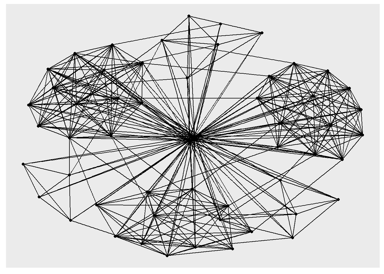

Fruchterman and Reingold layout

The code chunks below will be used to plot the network graph using Fruchterman and Reingold layout.

g <- ggraph(GAStech_graph, 
            layout = "fr") +
  geom_edge_link(aes()) +
  geom_node_point(aes())

g + theme_graph()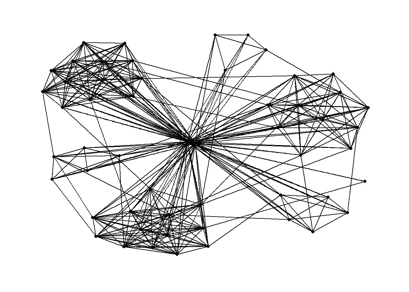

Modifying network nodes

In this section, you will colour each node by referring to their respective departments.

g <- ggraph(GAStech_graph, 
            layout = "nicely") + 
  geom_edge_link(aes()) +
  geom_node_point(aes(colour = Department, 
                      size = 3))

g + theme_graph()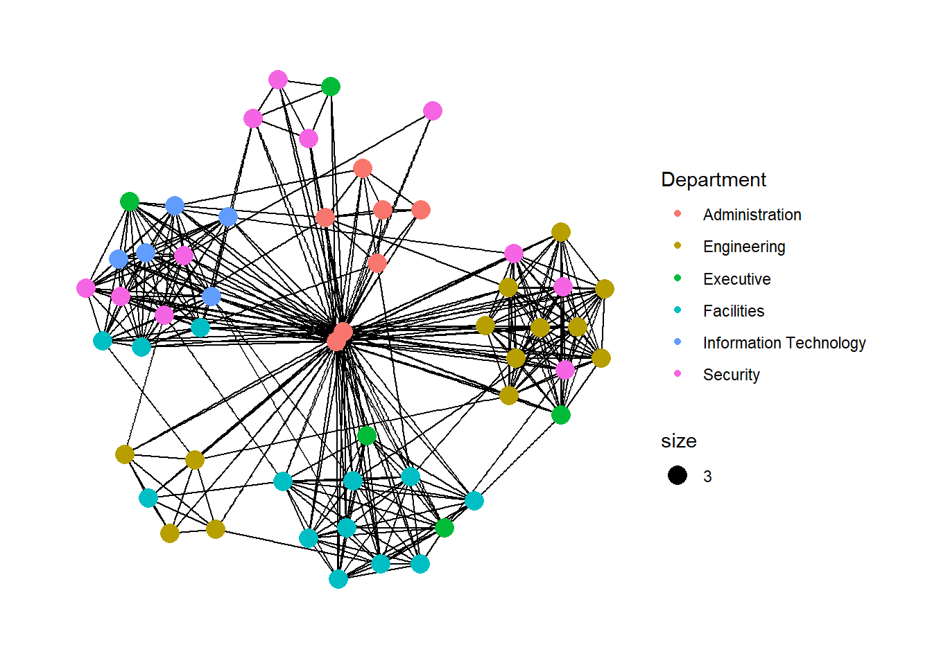

Modifying edges

In the code chunk below, the thickness of the edges will be mapped with the Weight variable.

g <- ggraph(GAStech_graph, 
            layout = "nicely") +
  geom_edge_link(aes(width=Weight), 
                 alpha=0.2) +
  scale_edge_width(range = c(0.1, 5)) +
  geom_node_point(aes(colour = Department), 
                  size = 3)

g + theme_graph()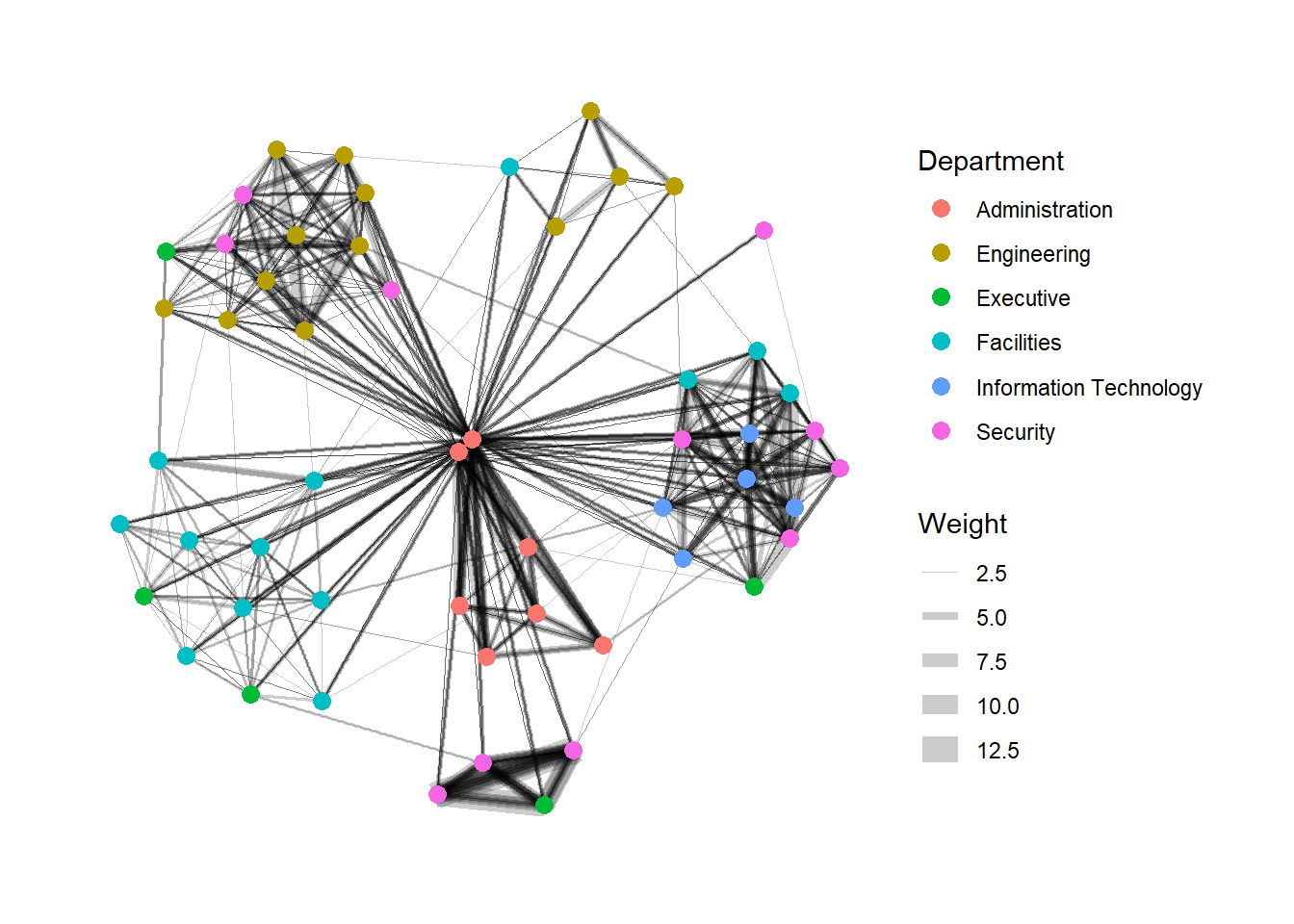

Working with facet_edges()

In the code chunk below, facet_edges() is used. Before getting started, it is advisable for you to read it’s reference guide at least once.

set_graph_style()

g <- ggraph(GAStech_graph, 
            layout = "nicely") + 
  geom_edge_link(aes(width=Weight), 
                 alpha=0.2) +
  scale_edge_width(range = c(0.1, 5)) +
  geom_node_point(aes(colour = Department), 
                  size = 2)

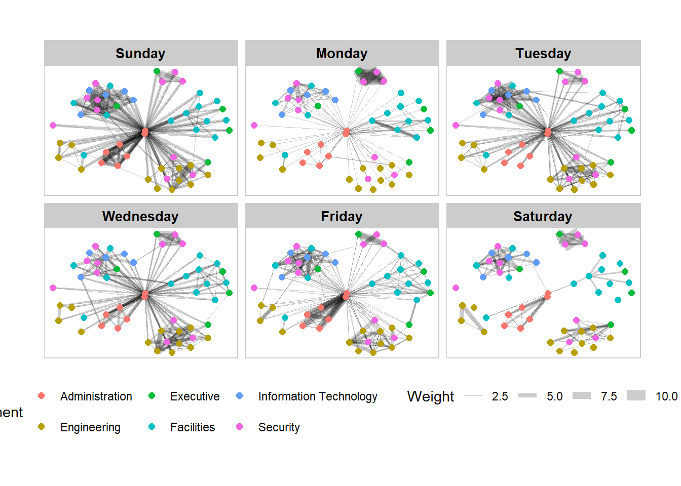
g + facet_edges(~Weekday)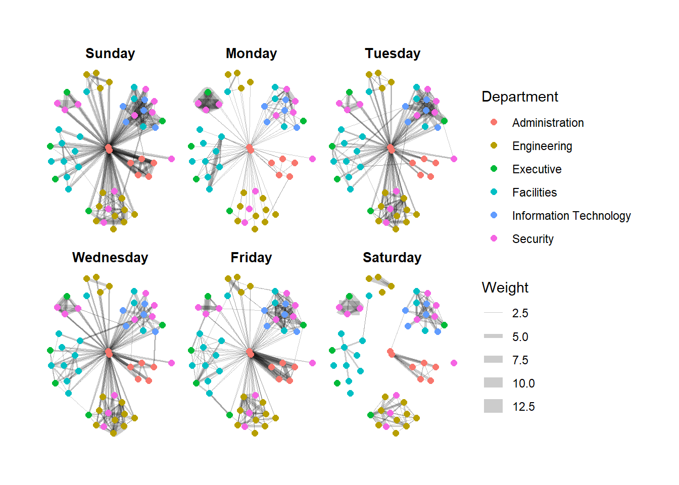

A framed facet graph

The code chunk below adds frame to each graph.

set_graph_style() 

g <- ggraph(GAStech_graph, 
            layout = "nicely") + 
  geom_edge_link(aes(width=Weight), 
                 alpha=0.2) +
  scale_edge_width(range = c(0.1, 5)) +
  geom_node_point(aes(colour = Department), 
                  size = 2)
  
g + facet_edges(~Weekday) +
  th_foreground(foreground = "grey80",  
                border = TRUE) +
  theme(legend.position = 'bottom')